W-types, fixed points and infinite structures
For as long as I have been interested in programming language theory, recursion (and its relationship with inductive data types) has always fascinated me. This whole conceptual area evokes the same feeling as that M.C. Escher drawing or The circular ruins story.
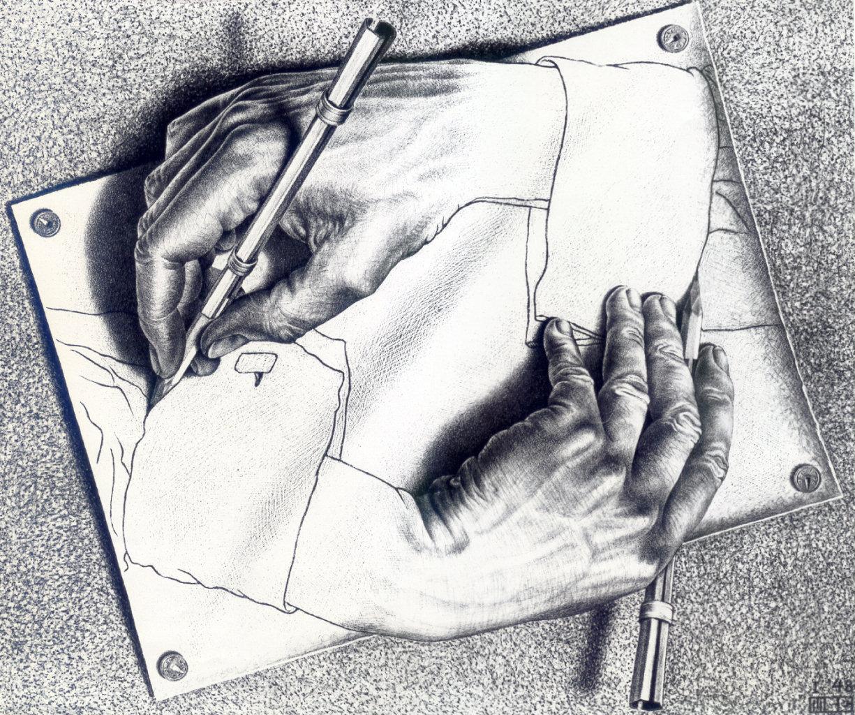
Everything seems to just be willed into existence simply by virtue of being consistent. This is confusing. In this post, I will attempt to ground those concepts and show that what looks like levitation11 See [1] is merely prestige.
module blog.fixpoints where
1. Simple types
Any good type systems is going to have, as its base layer, three things:
- Function types

- Product types

- Coproduct types

The function types are inhabited by our good old functions. We create functions by declaring arguments and stating how to use them to produce a result. We use function by applying them to arguments of the right type. All is as expected.
The product types are simply the family of things that are struct/tuple-like. They bind together data of different types. We construct elements of product types by giving data for each of the fields / components and we can use them by accessing the fields, either by name or by index. Again, this is standard stuff.
The coproduct types, on the other hand, are less well-known outside of functional programming languages and are also called sum types or tagged unions. They are named like this because the cardinality of a sum type is the sum of the cardinalities of its components. We construct an element of a sum type by giving a value for one of its components and we use a value from a sum type by pattern matching.
Once we add to our family the singleton type and the empty type22
You can also get there by defining your products and sums as  -ary
for any finite . In that case, the unit is the
-ary
for any finite . In that case, the unit is the  -ary product and
the empty type is the -ary sum.
, we end up
with what many people call “algebraic data types”. This is because if we adopt
isomorphism as the proper notion of equivalence of types, we get a ton of very
familiar mathematical identities.
-ary product and
the empty type is the -ary sum.
, we end up
with what many people call “algebraic data types”. This is because if we adopt
isomorphism as the proper notion of equivalence of types, we get a ton of very
familiar mathematical identities.

A calculus only armed with those types and the ability to name things can get us
surprisingly far. We can define booleans as  , then can
define all relevant operations through pattern matching and all is good. In
fact, we can construct a type with any finite number of elements. If we glue
this type system on top of the regular lambda calculus, we get the simply typed
lambda calculus, which has the nice properties that all programs terminate
(hence not Turing-complete). However, the language feels a bit unpractical,
notably for the absence of lists. Can we define lists exclusively through
products and sums? Almost. If we imagine for a moment the type of lists of
, then can
define all relevant operations through pattern matching and all is good. In
fact, we can construct a type with any finite number of elements. If we glue
this type system on top of the regular lambda calculus, we get the simply typed
lambda calculus, which has the nice properties that all programs terminate
(hence not Turing-complete). However, the language feels a bit unpractical,
notably for the absence of lists. Can we define lists exclusively through
products and sums? Almost. If we imagine for a moment the type of lists of  s. What shape can its element have? A list can be the empty list, or a
one-element list, or a two-element list, or a three-element list, and so on. In
fact, if our language of terms had a notion of “infinite sum”, we could define
lists as:
s. What shape can its element have? A list can be the empty list, or a
one-element list, or a two-element list, or a three-element list, and so on. In
fact, if our language of terms had a notion of “infinite sum”, we could define
lists as:

Sadly, our type system is too weak to be able to express these infinite sums. However, I propose that we adopt the “algebraic” point of view once again, squint a little and observe that the infinite sum can in fact be approached with a type-level “extend” operation:

If we apply it to the zero type, we get

If we apply it again, we get the type of lists with length  .
.

For each new layer of  we add, we get one new term of the
infinite sum.
we add, we get one new term of the
infinite sum.

It stands to reason that if we were able to ask from the type system “give me
the type that is applied an infinite number of times
to ”, then we would recover our beloved list type. In fact, because the
type of natural numbers can similarly be expressed as an infinite sum of ones

then we could also express natural numbers as the result of applying

an infinite number of times.
2. Inductive data types
It turns out, in fact, that the “apply this type function an infinite number of
times” operation is very close to the way most infinite data types are
understood in the theory. The main difference is that instead of talking about
infinite application, we talk about a fixed point. In mathematics, the fixpoint
of a function  is a value
  such that
  . This is
similar in spirit to our “infinite applications” formulation, because if there
were a value
. This is
similar in spirit to our “infinite applications” formulation, because if there
were a value  , then it would be a fixpoint because

We have motivated the need for a way to ask for fixpoint of type functions and
we want to apply this operation to and  . To achieve this, we will need to add a new primitive to
our language of types. Let us call this new primitive
. To achieve this, we will need to add a new primitive to
our language of types. Let us call this new primitive  .
.

Like we have done for the simple type, let us first start by defining the
language’s way to construct elements of this type; its introduction rule. Let  be a type-level function (like
  ), then from an element of
  , we can
construct an element of
, we can
construct an element of  using the
  function.

At first glance, it might look like creating a point of
requires us to have a point of . What sorcery! However,
it’s fine. If we look at  , the
, the  requirement turns out to
be easy to satisfy;
requirement turns out to
be easy to satisfy;

we can now easily construct an inhabitant of the left component.
At this point, we have a means to construct types with infinite elements. It might be tempting to define the elimination operator as simply the inverse of the introduction operator and call it a day.

Stop! while this  gives us the power of peeling any given
number of layers, it doesn’t let us peel an arbitrary number of layer.33
Up until now, I have implicitely assumed that the reader realizes our
object language doesn’t have recursion. This is implied by the fact we are
building on top of the simply typed lambda calculus (which doesn’t have it), but
it might be a useful reminder: we don’t have recursion, therefore
gives us the power of peeling any given
number of layers, it doesn’t let us peel an arbitrary number of layer.33
Up until now, I have implicitely assumed that the reader realizes our
object language doesn’t have recursion. This is implied by the fact we are
building on top of the simply typed lambda calculus (which doesn’t have it), but
it might be a useful reminder: we don’t have recursion, therefore  will always be called a bounded number of times. The elements
one is trying to deconstruct will go over this bound and bad stuff will happen.
For
that, we are going to define a second elimination operator.
will always be called a bounded number of times. The elements
one is trying to deconstruct will go over this bound and bad stuff will happen.
For
that, we are going to define a second elimination operator.

This type signature is weird. What does it feel to use it? Let’s use as an
example  , where we want to compute whether a list’s length
is even or odd. First, let’s specialize the
, where we want to compute whether a list’s length
is even or odd. First, let’s specialize the  operator to our
concrete types
operator to our
concrete types

For the first argument, we give the list we want to process and for the second,
some function which receives a  . Let’s call it
and look at what it sees. To use a sum, one must pattern match on the value. In
the case of our , that means considering two cases: one where it received
a unit
. Let’s call it
and look at what it sees. To use a sum, one must pattern match on the value. In
the case of our , that means considering two cases: one where it received
a unit  and another where it received a pair
  .
.

To see why returning  makes sense, let’s look at the
identity that provides a computational meaning to .
makes sense, let’s look at the
identity that provides a computational meaning to .

If, let’s say, a list has three elements, then it will be built out of four
layers of : one for each cons, one for the “base” empty list.

Applying our on that list would yield the following chain of equation

which is correct. Our operation has just introduced recursion
into our language. Even better, when we look at the type signature of  for the type function

we get primitive recursion. In fact, for lists also has a
known name: fold! Adding this single primitive to our type system has given us
access to types with infinite data, together with arbitrary finite
computation.44
There is an asterisk. For this to be true, we must only allow recursion
over when  is a strictly positive type functions.
There are other subtleties, but for the most part, this is
all I have to say for the non-dependent types case. Onto the next!55
There is still a lot of interesting stuff to know about those inductive
types. For instance, if our “type-level function” is viewed as a functor
in
is a strictly positive type functions.
There are other subtleties, but for the most part, this is
all I have to say for the non-dependent types case. Onto the next!55
There is still a lot of interesting stuff to know about those inductive
types. For instance, if our “type-level function” is viewed as a functor
in  , then the recursive data type
  can be
interpreted as the initial -algebra, where the initiality data is exactly
the existence of a operator. Fun stuff.
can be
interpreted as the initial -algebra, where the initiality data is exactly
the existence of a operator. Fun stuff.
3. Simple dependent types
If we take the simply typed lambda calculus and add all the axes of the lambda cube, we get the calculus of construction. In this calculus, the separation between the type language and the term language has vanished. A function can receive a value and return a type. A second function can receive a value and decide what type it will return based on the value. A function can take a type and return a value.66 Although this function would not be that useful, because of parametricity.
The type system of the calculus of constructions77 Or at least, the version I’m defining right here. is composed of two entities: pi types
![\[ \prod_{a : A} B(a) \]](data:image/svg+xml,%3C%3Fxml version=%271.0%27 encoding=%27UTF-8%27%3F%3E%0A%3C%21-- This file was generated by dvisvgm 3.4.3 --%3E%0A%3Csvg version=%271.1%27 xmlns=%27http://www.w3.org/2000/svg%27 xmlns:xlink=%27http://www.w3.org/1999/xlink%27 width=%27368.203724pt%27 height=%2725.856848pt%27 viewBox=%27-.500002 -25.356847 368.203724 25.856848%27%3E%0A%3Cdefs%3E%0A%3Cpath id=%27g10-40%27 d=%27m3.297634 2.391034c0-.029888 0-.049813-.169365-.219178c-1.24533-1.255293-1.564134-3.138232-1.564134-4.662516c0-1.733499 .37858-3.466999 1.603985-4.712329c.129514-.119552 .129514-.139477 .129514-.169365c0-.069738-.039851-.099626-.099626-.099626c-.099626 0-.996264 .67746-1.58406 1.942715c-.508095 1.09589-.627646 2.201743-.627646 3.038605c0 .777086 .109589 1.982565 .657534 3.108344c.597758 1.225405 1.454545 1.872976 1.554172 1.872976c.059776 0 .099626-.029888 .099626-.099626z%27/%3E%0A%3Cpath id=%27g10-41%27 d=%27m2.879203-2.49066c0-.777086-.109589-1.982565-.657534-3.108344c-.597758-1.225405-1.454545-1.872976-1.554172-1.872976c-.059776 0-.099626 .039851-.099626 .099626c0 .029888 0 .049813 .18929 .229141c.976339 .986301 1.544209 2.570361 1.544209 4.652553c0 1.703611-.368618 3.457036-1.603985 4.712329c-.129514 .119552-.129514 .139477-.129514 .169365c0 .059776 .039851 .099626 .099626 .099626c.099626 0 .996264-.67746 1.58406-1.942715c.508095-1.09589 .627646-2.201743 .627646-3.038605z%27/%3E%0A%3Cpath id=%27g8-66%27 d=%27m1.594022-.777086c-.099626 .388543-.119552 .468244-.9066 .468244c-.169365 0-.268991 0-.268991 .199253c0 .109589 .089664 .109589 .268991 .109589h3.556663c1.574097 0 2.749689-1.175592 2.749689-2.15193c0-.71731-.577833-1.295143-1.544209-1.404732c1.036115-.18929 2.082192-.926526 2.082192-1.872976c0-.737235-.657534-1.374844-1.853051-1.374844h-3.347447c-.18929 0-.288917 0-.288917 .199253c0 .109589 .089664 .109589 .278954 .109589c.019925 0 .209215 0 .37858 .019925c.179328 .019925 .268991 .029888 .268991 .159402c0 .039851-.009963 .069738-.039851 .18929l-1.334994 5.349938zm1.504359-2.86924l.617684-2.470735c.089664-.348692 .109589-.37858 .537983-.37858h1.285181c.876712 0 1.085928 .587796 1.085928 1.026152c0 .876712-.856787 1.823163-2.072229 1.823163h-1.454545zm-.448319 3.337484c-.139477 0-.159402 0-.219178-.009963c-.099626-.009963-.129514-.019925-.129514-.099626c0-.029888 0-.049813 .049813-.229141l.687422-2.779577h1.882939c.956413 0 1.145704 .737235 1.145704 1.165629c0 .986301-.886675 1.952677-2.062267 1.952677h-1.354919z%27/%3E%0A%3Cpath id=%27g8-97%27 d=%27m3.716065-3.765878c-.179328-.368618-.468244-.637609-.916563-.637609c-1.165629 0-2.400996 1.464508-2.400996 2.919054c0 .936488 .547945 1.594022 1.325031 1.594022c.199253 0 .697385-.039851 1.295143-.747198c.079701 .418431 .428394 .747198 .9066 .747198c.348692 0 .577833-.229141 .737235-.547945c.169365-.358655 .298879-.966376 .298879-.986301c0-.099626-.089664-.099626-.119552-.099626c-.099626 0-.109589 .039851-.139477 .179328c-.169365 .647572-.348692 1.235367-.757161 1.235367c-.268991 0-.298879-.259029-.298879-.458281c0-.219178 .019925-.298879 .129514-.737235c.109589-.418431 .129514-.518057 .219178-.896638l.358655-1.39477c.069738-.278954 .069738-.298879 .069738-.33873c0-.169365-.119552-.268991-.288917-.268991c-.239103 0-.388543 .219178-.418431 .438356zm-.647572 2.580324c-.049813 .179328-.049813 .199253-.199253 .368618c-.438356 .547945-.846824 .707347-1.125778 .707347c-.498132 0-.637609-.547945-.637609-.936488c0-.498132 .318804-1.723537 .547945-2.181818c.308842-.587796 .757161-.956413 1.155666-.956413c.647572 0 .787049 .816936 .787049 .876712s-.019925 .119552-.029888 .169365l-.498132 1.952677z%27/%3E%0A%3Cpath id=%27g11-58%27 d=%27m1.527273-2.601245c0-.244085-.195268-.404483-.397509-.404483c-.244085 0-.404483 .195268-.404483 .397509c0 .244085 .195268 .404483 .397509 .404483c.244085 0 .404483-.195268 .404483-.397509zm0 2.203736c0-.244085-.195268-.404483-.397509-.404483c-.244085 0-.404483 .195268-.404483 .397509c0 .244085 .195268 .404483 .397509 .404483c.244085 0 .404483-.195268 .404483-.397509z%27/%3E%0A%3Cpath id=%27g9-65%27 d=%27m1.436613-.836862c-.244085 .376588-.467248 .557908-.878705 .585803c-.069738 .006974-.160399 .006974-.160399 .146451c0 .076712 .062765 .104608 .097634 .104608c.18132 0 .411457-.027895 .599751-.027895c.223163 0 .509091 .027895 .718306 .027895c.034869 0 .139477 0 .139477-.153425c0-.09066-.09066-.097634-.118555-.097634c-.055791-.006974-.306849-.020922-.306849-.209215c0-.083686 .069738-.202242 .104608-.265006l.557908-.864757h1.994521l.167372 1.157659c-.027895 .069738-.069738 .18132-.481196 .18132c-.083686 0-.18132 0-.18132 .153425c0 .027895 .020922 .097634 .111582 .097634c.202242 0 .697385-.027895 .899626-.027895c.125529 0 .285928 .006974 .411457 .006974c.125529 .006974 .27198 .020922 .397509 .020922c.09066 0 .139477-.055791 .139477-.146451c0-.104608-.083686-.104608-.195268-.104608c-.404483 0-.418431-.055791-.439352-.223163l-.613699-4.302864c-.020922-.146451-.034869-.195268-.167372-.195268s-.174346 .062765-.237111 .160399l-2.559402 3.975093zm.920548-1.004234l1.464508-2.280448l.327771 2.280448h-1.792279z%27/%3E%0A%3Cpath id=%27g9-97%27 d=%27m2.942964-2.66401c-.146451-.230137-.383562-.411457-.718306-.411457c-.892653 0-1.799253 .983313-1.799253 1.987547c0 .676463 .4533 1.157659 1.053051 1.157659c.376588 0 .711333-.216189 .990286-.488169c.132503 .418431 .536986 .488169 .718306 .488169c.251059 0 .425405-.153425 .550934-.369614c.153425-.27198 .244085-.669489 .244085-.697385c0-.09066-.09066-.09066-.111582-.09066c-.097634 0-.104608 .027895-.153425 .216189c-.083686 .334745-.216189 .746202-.509091 .746202c-.18132 0-.230137-.153425-.230137-.341719c0-.118555 .055791-.369614 .104608-.550934c.048817-.188294 .118555-.474222 .153425-.627646l.139477-.530012c.041843-.18132 .125529-.509091 .125529-.54396c0-.153425-.125529-.223163-.237111-.223163c-.118555 0-.278954 .083686-.320797 .278954zm-.446326 1.792279c-.048817 .195268-.202242 .334745-.355666 .467248c-.062765 .055791-.341719 .278954-.641594 .278954c-.258032 0-.509091-.18132-.509091-.676463c0-.369614 .202242-1.136737 .36264-1.415691c.320797-.557908 .676463-.662516 .871731-.662516c.488169 0 .620672 .530012 .620672 .606725c0 .027895-.013948 .076712-.020922 .097634l-.327771 1.30411z%27/%3E%0A%3Cpath id=%27g12-89%27 d=%27m12.164384 13.947696v-.537983c-1.325031 0-1.633873-.458281-1.633873-1.09589v-10.67995c0-.647572 .318804-1.09589 1.633873-1.09589v-.537983h-11.606476v.537983c1.325031 0 1.633873 .458281 1.633873 1.09589v10.67995c0 .647572-.318804 1.09589-1.633873 1.09589v.537983h4.79203v-.537983c-1.325031 0-1.633873-.458281-1.633873-1.09589v-11.775841h5.290162v11.775841c0 .647572-.318804 1.09589-1.633873 1.09589v.537983h4.79203z%27/%3E%0A%3C/defs%3E%0A%3Cg id=%27page71%27%3E%0A%3Cg fill=%27currentColor%27%3E%0A%3Cuse x=%27165.870889%27 y=%27-22.366246%27 xlink:href=%27%23g12-89%27/%3E%0A%3Cuse x=%27165.951762%27 y=%27-.996264%27 xlink:href=%27%23g9-97%27/%3E%0A%3Cuse x=%27170.273206%27 y=%27-.996264%27 xlink:href=%27%23g11-58%27/%3E%0A%3Cuse x=%27172.528652%27 y=%27-.996264%27 xlink:href=%27%23g9-65%27/%3E%0A%3Cuse x=%27180.261352%27 y=%27-12.901677%27 xlink:href=%27%23g8-66%27/%3E%0A%3Cuse x=%27188.31796%27 y=%27-12.901677%27 xlink:href=%27%23g10-40%27/%3E%0A%3Cuse x=%27192.192334%27 y=%27-12.901677%27 xlink:href=%27%23g8-97%27/%3E%0A%3Cuse x=%27197.458488%27 y=%27-12.901677%27 xlink:href=%27%23g10-41%27/%3E%0A%3C/g%3E%0A%3C/g%3E%0A%3C/svg%3E)
and sigma types
![\[ \sum_{a : A} B(a) \]](data:image/svg+xml,%3C%3Fxml version=%271.0%27 encoding=%27UTF-8%27%3F%3E%0A%3C%21-- This file was generated by dvisvgm 3.4.3 --%3E%0A%3Csvg version=%271.1%27 xmlns=%27http://www.w3.org/2000/svg%27 xmlns:xlink=%27http://www.w3.org/1999/xlink%27 width=%27368.203724pt%27 height=%2725.856848pt%27 viewBox=%27-.500002 -25.356847 368.203724 25.856848%27%3E%0A%3Cdefs%3E%0A%3Cpath id=%27g10-40%27 d=%27m3.297634 2.391034c0-.029888 0-.049813-.169365-.219178c-1.24533-1.255293-1.564134-3.138232-1.564134-4.662516c0-1.733499 .37858-3.466999 1.603985-4.712329c.129514-.119552 .129514-.139477 .129514-.169365c0-.069738-.039851-.099626-.099626-.099626c-.099626 0-.996264 .67746-1.58406 1.942715c-.508095 1.09589-.627646 2.201743-.627646 3.038605c0 .777086 .109589 1.982565 .657534 3.108344c.597758 1.225405 1.454545 1.872976 1.554172 1.872976c.059776 0 .099626-.029888 .099626-.099626z%27/%3E%0A%3Cpath id=%27g10-41%27 d=%27m2.879203-2.49066c0-.777086-.109589-1.982565-.657534-3.108344c-.597758-1.225405-1.454545-1.872976-1.554172-1.872976c-.059776 0-.099626 .039851-.099626 .099626c0 .029888 0 .049813 .18929 .229141c.976339 .986301 1.544209 2.570361 1.544209 4.652553c0 1.703611-.368618 3.457036-1.603985 4.712329c-.129514 .119552-.129514 .139477-.129514 .169365c0 .059776 .039851 .099626 .099626 .099626c.099626 0 .996264-.67746 1.58406-1.942715c.508095-1.09589 .627646-2.201743 .627646-3.038605z%27/%3E%0A%3Cpath id=%27g8-66%27 d=%27m1.594022-.777086c-.099626 .388543-.119552 .468244-.9066 .468244c-.169365 0-.268991 0-.268991 .199253c0 .109589 .089664 .109589 .268991 .109589h3.556663c1.574097 0 2.749689-1.175592 2.749689-2.15193c0-.71731-.577833-1.295143-1.544209-1.404732c1.036115-.18929 2.082192-.926526 2.082192-1.872976c0-.737235-.657534-1.374844-1.853051-1.374844h-3.347447c-.18929 0-.288917 0-.288917 .199253c0 .109589 .089664 .109589 .278954 .109589c.019925 0 .209215 0 .37858 .019925c.179328 .019925 .268991 .029888 .268991 .159402c0 .039851-.009963 .069738-.039851 .18929l-1.334994 5.349938zm1.504359-2.86924l.617684-2.470735c.089664-.348692 .109589-.37858 .537983-.37858h1.285181c.876712 0 1.085928 .587796 1.085928 1.026152c0 .876712-.856787 1.823163-2.072229 1.823163h-1.454545zm-.448319 3.337484c-.139477 0-.159402 0-.219178-.009963c-.099626-.009963-.129514-.019925-.129514-.099626c0-.029888 0-.049813 .049813-.229141l.687422-2.779577h1.882939c.956413 0 1.145704 .737235 1.145704 1.165629c0 .986301-.886675 1.952677-2.062267 1.952677h-1.354919z%27/%3E%0A%3Cpath id=%27g8-97%27 d=%27m3.716065-3.765878c-.179328-.368618-.468244-.637609-.916563-.637609c-1.165629 0-2.400996 1.464508-2.400996 2.919054c0 .936488 .547945 1.594022 1.325031 1.594022c.199253 0 .697385-.039851 1.295143-.747198c.079701 .418431 .428394 .747198 .9066 .747198c.348692 0 .577833-.229141 .737235-.547945c.169365-.358655 .298879-.966376 .298879-.986301c0-.099626-.089664-.099626-.119552-.099626c-.099626 0-.109589 .039851-.139477 .179328c-.169365 .647572-.348692 1.235367-.757161 1.235367c-.268991 0-.298879-.259029-.298879-.458281c0-.219178 .019925-.298879 .129514-.737235c.109589-.418431 .129514-.518057 .219178-.896638l.358655-1.39477c.069738-.278954 .069738-.298879 .069738-.33873c0-.169365-.119552-.268991-.288917-.268991c-.239103 0-.388543 .219178-.418431 .438356zm-.647572 2.580324c-.049813 .179328-.049813 .199253-.199253 .368618c-.438356 .547945-.846824 .707347-1.125778 .707347c-.498132 0-.637609-.547945-.637609-.936488c0-.498132 .318804-1.723537 .547945-2.181818c.308842-.587796 .757161-.956413 1.155666-.956413c.647572 0 .787049 .816936 .787049 .876712s-.019925 .119552-.029888 .169365l-.498132 1.952677z%27/%3E%0A%3Cpath id=%27g11-58%27 d=%27m1.527273-2.601245c0-.244085-.195268-.404483-.397509-.404483c-.244085 0-.404483 .195268-.404483 .397509c0 .244085 .195268 .404483 .397509 .404483c.244085 0 .404483-.195268 .404483-.397509zm0 2.203736c0-.244085-.195268-.404483-.397509-.404483c-.244085 0-.404483 .195268-.404483 .397509c0 .244085 .195268 .404483 .397509 .404483c.244085 0 .404483-.195268 .404483-.397509z%27/%3E%0A%3Cpath id=%27g9-65%27 d=%27m1.436613-.836862c-.244085 .376588-.467248 .557908-.878705 .585803c-.069738 .006974-.160399 .006974-.160399 .146451c0 .076712 .062765 .104608 .097634 .104608c.18132 0 .411457-.027895 .599751-.027895c.223163 0 .509091 .027895 .718306 .027895c.034869 0 .139477 0 .139477-.153425c0-.09066-.09066-.097634-.118555-.097634c-.055791-.006974-.306849-.020922-.306849-.209215c0-.083686 .069738-.202242 .104608-.265006l.557908-.864757h1.994521l.167372 1.157659c-.027895 .069738-.069738 .18132-.481196 .18132c-.083686 0-.18132 0-.18132 .153425c0 .027895 .020922 .097634 .111582 .097634c.202242 0 .697385-.027895 .899626-.027895c.125529 0 .285928 .006974 .411457 .006974c.125529 .006974 .27198 .020922 .397509 .020922c.09066 0 .139477-.055791 .139477-.146451c0-.104608-.083686-.104608-.195268-.104608c-.404483 0-.418431-.055791-.439352-.223163l-.613699-4.302864c-.020922-.146451-.034869-.195268-.167372-.195268s-.174346 .062765-.237111 .160399l-2.559402 3.975093zm.920548-1.004234l1.464508-2.280448l.327771 2.280448h-1.792279z%27/%3E%0A%3Cpath id=%27g9-97%27 d=%27m2.942964-2.66401c-.146451-.230137-.383562-.411457-.718306-.411457c-.892653 0-1.799253 .983313-1.799253 1.987547c0 .676463 .4533 1.157659 1.053051 1.157659c.376588 0 .711333-.216189 .990286-.488169c.132503 .418431 .536986 .488169 .718306 .488169c.251059 0 .425405-.153425 .550934-.369614c.153425-.27198 .244085-.669489 .244085-.697385c0-.09066-.09066-.09066-.111582-.09066c-.097634 0-.104608 .027895-.153425 .216189c-.083686 .334745-.216189 .746202-.509091 .746202c-.18132 0-.230137-.153425-.230137-.341719c0-.118555 .055791-.369614 .104608-.550934c.048817-.188294 .118555-.474222 .153425-.627646l.139477-.530012c.041843-.18132 .125529-.509091 .125529-.54396c0-.153425-.125529-.223163-.237111-.223163c-.118555 0-.278954 .083686-.320797 .278954zm-.446326 1.792279c-.048817 .195268-.202242 .334745-.355666 .467248c-.062765 .055791-.341719 .278954-.641594 .278954c-.258032 0-.509091-.18132-.509091-.676463c0-.369614 .202242-1.136737 .36264-1.415691c.320797-.557908 .676463-.662516 .871731-.662516c.488169 0 .620672 .530012 .620672 .606725c0 .027895-.013948 .076712-.020922 .097634l-.327771 1.30411z%27/%3E%0A%3Cpath id=%27g12-88%27 d=%27m12.612702 13.947696l1.205479-3.188045h-.249066c-.388543 1.036115-1.444583 1.713574-2.590286 2.012453c-.209215 .049813-1.185554 .308842-3.098381 .308842h-6.007472l5.070984-5.947696c.069738-.079701 .089664-.109589 .089664-.159402c0-.019925 0-.049813-.069738-.14944l-4.64259-6.346202h5.459527c1.334994 0 2.241594 .139477 2.331258 .159402c.537983 .079701 1.404732 .249066 2.191781 .747198c.249066 .159402 .926526 .607721 1.265255 1.414695h.249066l-1.205479-2.799502h-11.775841c-.229141 0-.239103 .009963-.268991 .069738c-.009963 .029888-.009963 .219178-.009963 .328767l5.270237 7.212951l-5.160648 6.047323c-.099626 .119552-.099626 .169365-.099626 .179328c0 .109589 .089664 .109589 .268991 .109589h11.775841z%27/%3E%0A%3C/defs%3E%0A%3Cg id=%27page72%27%3E%0A%3Cg fill=%27currentColor%27%3E%0A%3Cuse x=%27165.040674%27 y=%27-22.366246%27 xlink:href=%27%23g12-88%27/%3E%0A%3Cuse x=%27165.951762%27 y=%27-.996264%27 xlink:href=%27%23g9-97%27/%3E%0A%3Cuse x=%27170.273206%27 y=%27-.996264%27 xlink:href=%27%23g11-58%27/%3E%0A%3Cuse x=%27172.528652%27 y=%27-.996264%27 xlink:href=%27%23g9-65%27/%3E%0A%3Cuse x=%27181.091582%27 y=%27-12.901677%27 xlink:href=%27%23g8-66%27/%3E%0A%3Cuse x=%27189.148191%27 y=%27-12.901677%27 xlink:href=%27%23g10-40%27/%3E%0A%3Cuse x=%27193.022564%27 y=%27-12.901677%27 xlink:href=%27%23g8-97%27/%3E%0A%3Cuse x=%27198.288718%27 y=%27-12.901677%27 xlink:href=%27%23g10-41%27/%3E%0A%3C/g%3E%0A%3C/g%3E%0A%3C/svg%3E)
Pi types, also known as dependent function types, are inhabited by functions and
are the generalization of both function types (as you would expect) and product
types (unlikely you would). You might see them in the wild denoted by  or, when the
  part is a constant w.r.t
  , by
, by  . The reason it generalizes over products is that under dependent types, a
function can hold exactly the information a product did in the STLC. For
instance, if a function takes in a boolean, it could choose to return a
. The reason it generalizes over products is that under dependent types, a
function can hold exactly the information a product did in the STLC. For
instance, if a function takes in a boolean, it could choose to return a  on
on  and something else on
  .
Functions therefore act like products where the sequence we are multiplying is
indexed by the domain of the function.
.
Functions therefore act like products where the sequence we are multiplying is
indexed by the domain of the function.
Sigma types, also known as dependent products are inhabited by variant-like data
and are the generalization of sum types. You might also see them denoted as  or, when the part is constant with respect to
  , by
, by  . The reason they generalize sums is that — like the
notation suggests – sigma types let you take the sum of a sequence of types
indexed by any type
. The reason they generalize sums is that — like the
notation suggests – sigma types let you take the sum of a sequence of types
indexed by any type  . In a way, they make the idea of tags even more
real, as they let you construct pairs where the type of the second component is
a function of the first component.
. In a way, they make the idea of tags even more
real, as they let you construct pairs where the type of the second component is
a function of the first component.
Again, we can add to our family the empty type , then construct the unit
type as the pi type  with empty
codomain. We end up in a situation that is very similar to the one we were in
with the simply typed lambda calculus. We have no way of constructing infinite
data types like lists or natural numbers!
with empty
codomain. We end up in a situation that is very similar to the one we were in
with the simply typed lambda calculus. We have no way of constructing infinite
data types like lists or natural numbers!
A first idea might be to add back in. After all, the calculus
of constructions is a super set of the simply typed lambda calculus, therefore
it is probably compatible with the nice extension we came up earlier. Doing that
half works. On one hand, we recover the nice types and recursion we had
earlier, but in the context of dependent types, they now appear severely
underpowered.
The first thing we can do is try and extend the eliminator to
enable expressing this type of function. Let’s recall the type signature of our
old operator, with all the type paramers made explicit arguments:88
This is possible, again, because in dependent type theory, functions can
take as arguments a mix of types and values.

We want to tweak it until it does what we want: return values of types that
depend on the input value. The obvious (because it is necessary) thing to do is
express the return type  as a function of the input.

Here, we have the right shape, but it is still unclear what should go into the
hole. We know it should look at an whose branch contain  , but because cannot have branches with different
types, the current formulation is simply incompatible with dependent
elimination. It turns out that we will need to move to a different fixpoint
primitve altogether if we want to have a single new primitive give us the whole
package.99
Something type theories often do is define introduction and elimination
rules ad hoc for all inductive types. If we did that, we would have a intro/elim
pair for lists, one for naturals, et cetera. Because we want to have a closed
type theory that does everything we want directly, we will instead work towards
a single primitive that let us implement all inductive types.
, but because cannot have branches with different
types, the current formulation is simply incompatible with dependent
elimination. It turns out that we will need to move to a different fixpoint
primitve altogether if we want to have a single new primitive give us the whole
package.99
Something type theories often do is define introduction and elimination
rules ad hoc for all inductive types. If we did that, we would have a intro/elim
pair for lists, one for naturals, et cetera. Because we want to have a closed
type theory that does everything we want directly, we will instead work towards
a single primitive that let us implement all inductive types.
4. W-types
W types are something like a generalization of that let us do
dependent elimination. As a bonus, it also gives us access to a new family of
inductive types: the infinitary trees.
A W-type is defined through a single type constructor  .1010
You should note that W-types are essentially the same thing as what
people, later, begin to call “container”. In [2], they show that
these containers correspond exactly to what we think of as “strictly
positive/polynomial functors”.
.1010
You should note that W-types are essentially the same thing as what
people, later, begin to call “container”. In [2], they show that
these containers correspond exactly to what we think of as “strictly
positive/polynomial functors”.

Here, the first argument  is a type whose elements represent the
different labels (think of them as node types) of your tree data type. The
second argument
is a type whose elements represent the
different labels (think of them as node types) of your tree data type. The
second argument  (for “branches”) takes a label and give you a type with
as many element as there are children under that node. This is where the
infinitary property comes in. If
(for “branches”) takes a label and give you a type with
as many element as there are children under that node. This is where the
infinitary property comes in. If  evaluates to a type with infinite
elements, then nodes with label
evaluates to a type with infinite
elements, then nodes with label  will have infinite direct children. Now
let’s look at the introduction rule:
will have infinite direct children. Now
let’s look at the introduction rule:

From top to bottom: the first two arguments are the parameters of the  type constructor itself. Then, is the label of the node we
are trying to create. Finally, the
type constructor itself. Then, is the label of the node we
are trying to create. Finally, the  function associates
to each child slot a child node. The eliminator then has the following type
signature.
function associates
to each child slot a child node. The eliminator then has the following type
signature.
![\begin{align*}
\mathsf{ind} &: (L : \mathsf{Type}) \\
&\to (B : L \to \mathsf{Type}) \\
&\to (M : \mathsf{W}(L, B) \to \mathsf{Type}) \\
&\to \begin{aligned}[t] (&(l : L) \to (c : (b : B(l)) \to \mathsf{W}(L, B)) \\
&\to (r : (b : B(l)) \to M(c(b))) \\
&\to M(\mathsf{cons}(L, B, l, c)))
\end{aligned} \\
&\to (w : \mathsf{W}(L,B)) \\
&\to M(w)
\end{align*}](data:image/svg+xml,%3C%3Fxml version=%271.0%27 encoding=%27UTF-8%27%3F%3E%0A%3C%21-- This file was generated by dvisvgm 3.4.3 --%3E%0A%3Csvg version=%271.1%27 xmlns=%27http://www.w3.org/2000/svg%27 xmlns:xlink=%27http://www.w3.org/1999/xlink%27 width=%27368.203724pt%27 height=%27122.145744pt%27 viewBox=%27-.500002 -118.059155 368.203724 122.145744%27%3E%0A%3Cdefs%3E%0A%3Cpath id=%27g1-33%27 d=%27m8.308842-2.291407c-.547945 .418431-.816936 .826899-.896638 .956413c-.448319 .687422-.52802 1.315068-.52802 1.325031c0 .119552 .119552 .119552 .199253 .119552c.169365 0 .179328-.019925 .219178-.199253c.229141-.976339 .816936-1.8132 1.942715-2.271482c.119552-.039851 .14944-.059776 .14944-.129514s-.059776-.099626-.079701-.109589c-.438356-.169365-1.643836-.667497-2.022416-2.34122c-.029888-.119552-.039851-.14944-.209215-.14944c-.079701 0-.199253 0-.199253 .119552c0 .019925 .089664 .647572 .508095 1.315068c.199253 .298879 .488169 .647572 .916563 .966376h-7.402242c-.179328 0-.358655 0-.358655 .199253s.179328 .199253 .358655 .199253h7.402242z%27/%3E%0A%3Cpath id=%27g2-59%27 d=%27m2.022416-.009963c0-.657534-.249066-1.046077-.637609-1.046077c-.328767 0-.52802 .249066-.52802 .52802c0 .268991 .199253 .52802 .52802 .52802c.119552 0 .249066-.039851 .348692-.129514c.029888-.019925 .039851-.029888 .049813-.029888s.019925 .009963 .019925 .14944c0 .737235-.348692 1.334994-.67746 1.663761c-.109589 .109589-.109589 .129514-.109589 .159402c0 .069738 .049813 .109589 .099626 .109589c.109589 0 .9066-.767123 .9066-1.932752z%27/%3E%0A%3Cpath id=%27g2-66%27 d=%27m1.594022-.777086c-.099626 .388543-.119552 .468244-.9066 .468244c-.169365 0-.268991 0-.268991 .199253c0 .109589 .089664 .109589 .268991 .109589h3.556663c1.574097 0 2.749689-1.175592 2.749689-2.15193c0-.71731-.577833-1.295143-1.544209-1.404732c1.036115-.18929 2.082192-.926526 2.082192-1.872976c0-.737235-.657534-1.374844-1.853051-1.374844h-3.347447c-.18929 0-.288917 0-.288917 .199253c0 .109589 .089664 .109589 .278954 .109589c.019925 0 .209215 0 .37858 .019925c.179328 .019925 .268991 .029888 .268991 .159402c0 .039851-.009963 .069738-.039851 .18929l-1.334994 5.349938zm1.504359-2.86924l.617684-2.470735c.089664-.348692 .109589-.37858 .537983-.37858h1.285181c.876712 0 1.085928 .587796 1.085928 1.026152c0 .876712-.856787 1.823163-2.072229 1.823163h-1.454545zm-.448319 3.337484c-.139477 0-.159402 0-.219178-.009963c-.099626-.009963-.129514-.019925-.129514-.099626c0-.029888 0-.049813 .049813-.229141l.687422-2.779577h1.882939c.956413 0 1.145704 .737235 1.145704 1.165629c0 .986301-.886675 1.952677-2.062267 1.952677h-1.354919z%27/%3E%0A%3Cpath id=%27g2-76%27 d=%27m3.726027-6.027397c.089664-.358655 .119552-.468244 1.05604-.468244c.298879 0 .37858 0 .37858-.18929c0-.119552-.109589-.119552-.159402-.119552c-.328767 0-1.145704 .029888-1.474471 .029888c-.298879 0-1.026152-.029888-1.325031-.029888c-.069738 0-.18929 0-.18929 .199253c0 .109589 .089664 .109589 .278954 .109589c.019925 0 .209215 0 .37858 .019925c.179328 .019925 .268991 .029888 .268991 .159402c0 .039851-.009963 .069738-.039851 .18929l-1.334994 5.349938c-.099626 .388543-.119552 .468244-.9066 .468244c-.169365 0-.268991 0-.268991 .199253c0 .109589 .089664 .109589 .268991 .109589h4.612702c.239103 0 .249066 0 .308842-.169365l.787049-2.15193c.039851-.109589 .039851-.129514 .039851-.139477c0-.039851-.029888-.109589-.119552-.109589s-.099626 .049813-.169365 .209215c-.33873 .916563-.777086 2.052304-2.500623 2.052304h-.936488c-.139477 0-.159402 0-.219178-.009963c-.099626-.009963-.129514-.019925-.129514-.099626c0-.029888 0-.049813 .049813-.229141l1.344956-5.379826z%27/%3E%0A%3Cpath id=%27g2-77%27 d=%27m9.225405-6.03736c.089664-.358655 .109589-.458281 .856787-.458281c.229141 0 .318804 0 .318804-.199253c0-.109589-.099626-.109589-.268991-.109589h-1.315068c-.259029 0-.268991 0-.388543 .18929l-3.636364 5.678705l-.777086-5.638854c-.029888-.229141-.049813-.229141-.308842-.229141h-1.364882c-.18929 0-.298879 0-.298879 .18929c0 .119552 .089664 .119552 .288917 .119552c.129514 0 .308842 .009963 .428394 .019925c.159402 .019925 .219178 .049813 .219178 .159402c0 .039851-.009963 .069738-.039851 .18929l-1.265255 5.070984c-.099626 .398506-.268991 .71731-1.075965 .747198c-.049813 0-.179328 .009963-.179328 .18929c0 .089664 .059776 .119552 .139477 .119552c.318804 0 .667497-.029888 .996264-.029888c.33873 0 .697385 .029888 1.026152 .029888c.049813 0 .179328 0 .179328-.199253c0-.109589-.109589-.109589-.179328-.109589c-.56787-.009963-.67746-.209215-.67746-.438356c0-.069738 .009963-.119552 .039851-.229141l1.354919-5.429639h.009963l.856787 6.176837c.019925 .119552 .029888 .229141 .14944 .229141c.109589 0 .169365-.109589 .219178-.179328l4.024907-6.306351h.009963l-1.424658 5.708593c-.099626 .388543-.119552 .468244-.9066 .468244c-.169365 0-.278954 0-.278954 .18929c0 .119552 .119552 .119552 .14944 .119552c.278954 0 .956413-.029888 1.235367-.029888c.408468 0 .836862 .029888 1.24533 .029888c.059776 0 .18929 0 .18929-.199253c0-.109589-.089664-.109589-.278954-.109589c-.368618 0-.647572 0-.647572-.179328c0-.039851 0-.059776 .049813-.239103l1.325031-5.310087z%27/%3E%0A%3Cpath id=%27g2-98%27 d=%27m2.381071-6.804483c0-.009963 0-.109589-.129514-.109589c-.229141 0-.956413 .079701-1.215442 .099626c-.079701 .009963-.18929 .019925-.18929 .199253c0 .119552 .089664 .119552 .239103 .119552c.478207 0 .498132 .069738 .498132 .169365c0 .069738-.089664 .408468-.139477 .617684l-.816936 3.247821c-.119552 .498132-.159402 .657534-.159402 1.006227c0 .946451 .52802 1.564134 1.265255 1.564134c1.175592 0 2.400996-1.484433 2.400996-2.919054c0-.9066-.52802-1.594022-1.325031-1.594022c-.458281 0-.86675 .288917-1.165629 .597758l.737235-2.998755zm-.936488 3.765878c.059776-.219178 .059776-.239103 .14944-.348692c.488169-.647572 .936488-.797011 1.195517-.797011c.358655 0 .627646 .298879 .627646 .936488c0 .587796-.328767 1.733499-.508095 2.11208c-.328767 .667497-.787049 1.026152-1.175592 1.026152c-.33873 0-.667497-.268991-.667497-1.006227c0-.18929 0-.37858 .159402-1.006227l.219178-.916563z%27/%3E%0A%3Cpath id=%27g2-99%27 d=%27m3.945205-3.785803c-.159402 0-.298879 0-.438356 .139477c-.159402 .14944-.179328 .318804-.179328 .388543c0 .239103 .179328 .348692 .368618 .348692c.288917 0 .557908-.239103 .557908-.637609c0-.488169-.468244-.856787-1.175592-.856787c-1.344956 0-2.669988 1.424658-2.669988 2.82939c0 .896638 .577833 1.683686 1.613948 1.683686c1.424658 0 2.261519-1.05604 2.261519-1.175592c0-.059776-.059776-.129514-.119552-.129514c-.049813 0-.069738 .019925-.129514 .099626c-.787049 .986301-1.872976 .986301-1.992528 .986301c-.627646 0-.896638-.488169-.896638-1.085928c0-.408468 .199253-1.374844 .537983-1.992528c.308842-.56787 .856787-.996264 1.404732-.996264c.33873 0 .71731 .129514 .856787 .398506z%27/%3E%0A%3Cpath id=%27g2-108%27 d=%27m2.570361-6.804483c0-.009963 0-.109589-.129514-.109589c-.229141 0-.956413 .079701-1.215442 .099626c-.079701 .009963-.18929 .019925-.18929 .209215c0 .109589 .099626 .109589 .249066 .109589c.478207 0 .488169 .089664 .488169 .169365l-.029888 .199253l-1.255293 4.98132c-.029888 .109589-.049813 .179328-.049813 .33873c0 .56787 .438356 .916563 .9066 .916563c.328767 0 .577833-.199253 .747198-.557908c.179328-.37858 .298879-.956413 .298879-.976339c0-.099626-.089664-.099626-.119552-.099626c-.099626 0-.109589 .039851-.139477 .179328c-.169365 .647572-.358655 1.235367-.757161 1.235367c-.298879 0-.298879-.318804-.298879-.458281c0-.239103 .009963-.288917 .059776-.478207l1.43462-5.758406z%27/%3E%0A%3Cpath id=%27g2-114%27 d=%27m.876712-.587796c-.029888 .14944-.089664 .37858-.089664 .428394c0 .179328 .139477 .268991 .288917 .268991c.119552 0 .298879-.079701 .368618-.278954c.019925-.039851 .358655-1.39477 .398506-1.574097c.079701-.328767 .259029-1.026152 .318804-1.295143c.039851-.129514 .318804-.597758 .557908-.816936c.079701-.069738 .368618-.328767 .797011-.328767c.259029 0 .408468 .119552 .418431 .119552c-.298879 .049813-.518057 .288917-.518057 .547945c0 .159402 .109589 .348692 .37858 .348692s.547945-.229141 .547945-.587796c0-.348692-.318804-.647572-.826899-.647572c-.647572 0-1.085928 .488169-1.275218 .767123c-.079701-.448319-.438356-.767123-.9066-.767123c-.458281 0-.647572 .388543-.737235 .56787c-.179328 .33873-.308842 .936488-.308842 .966376c0 .099626 .099626 .099626 .119552 .099626c.099626 0 .109589-.009963 .169365-.229141c.169365-.707347 .368618-1.185554 .727273-1.185554c.169365 0 .308842 .079701 .308842 .458281c0 .209215-.029888 .318804-.159402 .836862l-.577833 2.30137z%27/%3E%0A%3Cpath id=%27g2-119%27 d=%27m4.60274-3.377335c.049813-.219178 .14944-.587796 .14944-.647572c0-.179328-.139477-.268991-.288917-.268991c-.119552 0-.298879 .079701-.368618 .278954c-.029888 .069738-.498132 1.972603-.56787 2.231631c-.069738 .298879-.089664 .478207-.089664 .657534c0 .109589 0 .129514 .009963 .179328c-.229141 .52802-.52802 .836862-.916563 .836862c-.797011 0-.797011-.737235-.797011-.9066c0-.318804 .049813-.707347 .518057-1.932752c.109589-.298879 .169365-.438356 .169365-.637609c0-.448319-.328767-.816936-.816936-.816936c-.946451 0-1.315068 1.444583-1.315068 1.534247c0 .099626 .099626 .099626 .119552 .099626c.099626 0 .109589-.019925 .159402-.179328c.268991-.926526 .657534-1.235367 1.006227-1.235367c.089664 0 .249066 .009963 .249066 .328767c0 .249066-.109589 .52802-.179328 .697385c-.438356 1.175592-.557908 1.633873-.557908 2.012453c0 .9066 .667497 1.255293 1.414695 1.255293c.169365 0 .637609 0 1.036115-.697385c.259029 .637609 .946451 .697385 1.24533 .697385c.747198 0 1.185554-.627646 1.444583-1.225405c.33873-.777086 .657534-2.11208 .657534-2.590286c0-.547945-.268991-.697385-.438356-.697385c-.249066 0-.498132 .259029-.498132 .478207c0 .129514 .059776 .18929 .14944 .268991c.109589 .109589 .358655 .368618 .358655 .846824c0 .33873-.288917 1.315068-.547945 1.823163c-.259029 .52802-.607721 .876712-1.09589 .876712c-.468244 0-.737235-.298879-.737235-.86675c0-.278954 .069738-.587796 .109589-.727273l.418431-1.673724z%27/%3E%0A%3Cpath id=%27g3-40%27 d=%27m3.297634 2.391034c0-.029888 0-.049813-.169365-.219178c-1.24533-1.255293-1.564134-3.138232-1.564134-4.662516c0-1.733499 .37858-3.466999 1.603985-4.712329c.129514-.119552 .129514-.139477 .129514-.169365c0-.069738-.039851-.099626-.099626-.099626c-.099626 0-.996264 .67746-1.58406 1.942715c-.508095 1.09589-.627646 2.201743-.627646 3.038605c0 .777086 .109589 1.982565 .657534 3.108344c.597758 1.225405 1.454545 1.872976 1.554172 1.872976c.059776 0 .099626-.029888 .099626-.099626z%27/%3E%0A%3Cpath id=%27g3-41%27 d=%27m2.879203-2.49066c0-.777086-.109589-1.982565-.657534-3.108344c-.597758-1.225405-1.454545-1.872976-1.554172-1.872976c-.059776 0-.099626 .039851-.099626 .099626c0 .029888 0 .049813 .18929 .229141c.976339 .986301 1.544209 2.570361 1.544209 4.652553c0 1.703611-.368618 3.457036-1.603985 4.712329c-.129514 .119552-.129514 .139477-.129514 .169365c0 .059776 .039851 .099626 .099626 .099626c.099626 0 .996264-.67746 1.58406-1.942715c.508095-1.09589 .627646-2.201743 .627646-3.038605z%27/%3E%0A%3Cpath id=%27g3-58%27 d=%27m1.912827-3.765878c0-.288917-.239103-.52802-.52802-.52802s-.52802 .239103-.52802 .52802s.239103 .52802 .52802 .52802s.52802-.239103 .52802-.52802zm0 3.237858c0-.288917-.239103-.52802-.52802-.52802s-.52802 .239103-.52802 .52802s.239103 .52802 .52802 .52802s.52802-.239103 .52802-.52802z%27/%3E%0A%3Cpath id=%27g0-84%27 d=%27m3.835616-6.216687h.886675c.119552 0 .239103 .009963 .358655 .009963h1.334994v-.647572h-6.057285v.647572h1.334994c.119552 0 .239103-.009963 .358655-.009963h.896638v6.216687h.886675v-6.216687z%27/%3E%0A%3Cpath id=%27g0-87%27 d=%27m9.255293-6.914072h-.71731l-.9066 3.128269c-.259029 .886675-.737235 2.560399-.787049 3.068493h-.009963c0-.009963-.059776-.52802-.71731-2.799502l-.976339-3.39726h-.806974l-.896638 3.108344c-.219178 .767123-.71731 2.510585-.767123 3.068493h-.009963c-.039851-.398506-.308842-1.374844-.388543-1.703611l-.468244-1.663761l-.806974-2.809465h-.856787l2.022416 6.914072h.806974l.996264-3.457036c.209215-.727273 .637609-2.211706 .697385-2.729763h.009963c.039851 .298879 .278954 1.24533 .547945 2.191781l1.145704 3.995019h.86675l2.022416-6.914072z%27/%3E%0A%3Cpath id=%27g0-99%27 d=%27m4.084682-4.164384c-.587796-.33873-.926526-.428394-1.534247-.428394c-1.384807 0-2.191781 1.205479-2.191781 2.381071c0 1.235367 .9066 2.321295 2.15193 2.321295c.537983 0 1.085928-.139477 1.62391-.508095l-.059776-.667497c-.508095 .398506-1.046077 .537983-1.554172 .537983c-.826899 0-1.384807-.71731-1.384807-1.693649c0-.777086 .368618-1.733499 1.424658-1.733499c.518057 0 .856787 .079701 1.404732 .438356l.119552-.647572z%27/%3E%0A%3Cpath id=%27g0-100%27 d=%27m4.323786-6.914072h-.747198v2.929016c-.52802-.438356-1.085928-.547945-1.454545-.547945c-.986301 0-1.763387 1.036115-1.763387 2.321295c0 1.305106 .767123 2.321295 1.713574 2.321295c.328767 0 .916563-.089664 1.474471-.627646v.518057h.777086v-6.914072zm-.777086 5.529265c0 .139477-.009963 .318804-.328767 .607721c-.229141 .199253-.478207 .278954-.737235 .278954c-.617684 0-1.344956-.468244-1.344956-1.703611c0-1.315068 .856787-1.723537 1.444583-1.723537c.448319 0 .747198 .229141 .966376 .547945v1.992528z%27/%3E%0A%3Cpath id=%27g0-101%27 d=%27m4.124533-2.181818c0-.33873-.009963-1.085928-.398506-1.683686c-.408468-.617684-1.016189-.727273-1.374844-.727273c-1.105853 0-2.002491 1.05604-2.002491 2.34122c0 1.315068 .956413 2.361146 2.15193 2.361146c.627646 0 1.195517-.239103 1.58406-.518057l-.059776-.647572c-.627646 .518057-1.285181 .557908-1.514321 .557908c-.797011 0-1.43462-.707347-1.464508-1.683686h3.078456zm-3.028643-.547945c.159402-.757161 .687422-1.255293 1.255293-1.255293c.518057 0 1.075965 .33873 1.205479 1.255293h-2.460772z%27/%3E%0A%3Cpath id=%27g0-105%27 d=%27m1.62391-6.774595h-.886675v.886675h.886675v-.886675zm-.069738 2.351183h-.747198v4.423412h.747198v-4.423412z%27/%3E%0A%3Cpath id=%27g0-110%27 d=%27m4.333748-2.968867c0-.657534-.14944-1.564134-1.364882-1.564134c-.896638 0-1.384807 .67746-1.444583 .757161v-.707347h-.71731v4.483188h.777086v-2.440847c0-.657534 .249066-1.484433 1.006227-1.484433c.956413 0 .966376 .707347 .966376 1.026152v2.899128h.777086v-2.968867z%27/%3E%0A%3Cpath id=%27g0-111%27 d=%27m4.672478-2.191781c0-1.334994-.996264-2.400996-2.181818-2.400996c-1.225405 0-2.191781 1.09589-2.191781 2.400996c0 1.315068 1.016189 2.30137 2.181818 2.30137c1.195517 0 2.191781-1.006227 2.191781-2.30137zm-2.191781 1.663761c-.687422 0-1.404732-.557908-1.404732-1.763387s.757161-1.693649 1.404732-1.693649c.697385 0 1.414695 .518057 1.414695 1.693649s-.67746 1.763387-1.414695 1.763387z%27/%3E%0A%3Cpath id=%27g0-112%27 d=%27m1.594022-.458281c.308842 .288917 .747198 .56787 1.344956 .56787c.966376 0 1.843088-.976339 1.843088-2.331258c0-1.195517-.627646-2.311333-1.58406-2.311333c-.597758 0-1.175592 .209215-1.633873 .597758v-.488169h-.747198v6.356164h.777086v-2.391034zm0-2.859278c.239103-.348692 .627646-.577833 1.05604-.577833c.757161 0 1.354919 .757161 1.354919 1.673724c0 1.026152-.707347 1.723537-1.454545 1.723537c-.388543 0-.657534-.199253-.856787-.468244c-.099626-.14944-.099626-.169365-.099626-.348692v-2.002491z%27/%3E%0A%3Cpath id=%27g0-115%27 d=%27m3.417186-4.273973c-.518057-.239103-.926526-.318804-1.43462-.318804c-.249066 0-1.653798 0-1.653798 1.305106c0 .488169 .288917 .806974 .537983 .996264c.308842 .219178 .52802 .259029 1.075965 .368618c.358655 .069738 .936488 .18929 .936488 .71731c0 .687422-.787049 .687422-.936488 .687422c-.806974 0-1.364882-.368618-1.544209-.488169l-.119552 .67746c.318804 .159402 .86675 .438356 1.673724 .438356c.179328 0 .727273 0 1.155666-.318804c.308842-.239103 .478207-.637609 .478207-1.066002c0-.547945-.368618-.886675-.388543-.916563c-.388543-.348692-.657534-.408468-1.155666-.498132c-.547945-.109589-1.006227-.209215-1.006227-.697385c0-.617684 .71731-.617684 .846824-.617684c.318804 0 .846824 .039851 1.414695 .37858l.119552-.647572z%27/%3E%0A%3Cpath id=%27g0-121%27 d=%27m4.443337-4.423412h-.747198c-1.295143 3.16812-1.315068 3.626401-1.325031 3.855542h-.009963c-.059776-.667497-.856787-2.520548-.896638-2.610212l-.537983-1.24533h-.787049l1.932752 4.423412c-.119552 .308842-.318804 .806974-.358655 .896638c-.259029 .577833-.428394 .577833-.56787 .577833c-.159402 0-.478207-.039851-.777086-.159402l.059776 .647572c.219178 .049813 .498132 .079701 .71731 .079701c.348692 0 .71731-.119552 1.125778-1.135741l2.171856-5.330012z%27/%3E%0A%3C/defs%3E%0A%3Cg id=%27page2%27%3E%0A%3Cuse x=%2790.969761%27 y=%27-105.603985%27 xlink:href=%27%23g0-105%27/%3E%0A%3Cuse x=%2793.349733%27 y=%27-105.603985%27 xlink:href=%27%23g0-110%27/%3E%0A%3Cuse x=%2798.497114%27 y=%27-105.603985%27 xlink:href=%27%23g0-100%27/%3E%0A%3Cuse x=%27106.411793%27 y=%27-105.603985%27 xlink:href=%27%23g3-58%27/%3E%0A%3Cuse x=%27111.946534%27 y=%27-105.603985%27 xlink:href=%27%23g3-40%27/%3E%0A%3Cuse x=%27115.820907%27 y=%27-105.603985%27 xlink:href=%27%23g2-76%27/%3E%0A%3Cuse x=%27125.368387%27 y=%27-105.603985%27 xlink:href=%27%23g3-58%27/%3E%0A%3Cuse x=%27130.903128%27 y=%27-105.603985%27 xlink:href=%27%23g0-84%27/%3E%0A%3Cuse x=%27136.853044%27 y=%27-105.603985%27 xlink:href=%27%23g0-121%27/%3E%0A%3Cuse x=%27141.446947%27 y=%27-105.603985%27 xlink:href=%27%23g0-112%27/%3E%0A%3Cuse x=%27146.871076%27 y=%27-105.603985%27 xlink:href=%27%23g0-101%27/%3E%0A%3Cuse x=%27151.298903%27 y=%27-105.603985%27 xlink:href=%27%23g3-41%27/%3E%0A%3Cuse x=%27106.411793%27 y=%27-90.660025%27 xlink:href=%27%23g1-33%27/%3E%0A%3Cuse x=%27119.141794%27 y=%27-90.660025%27 xlink:href=%27%23g3-40%27/%3E%0A%3Cuse x=%27123.016167%27 y=%27-90.660025%27 xlink:href=%27%23g2-66%27/%3E%0A%3Cuse x=%27133.840108%27 y=%27-90.660025%27 xlink:href=%27%23g3-58%27/%3E%0A%3Cuse x=%27139.374849%27 y=%27-90.660025%27 xlink:href=%27%23g2-76%27/%3E%0A%3Cuse x=%27148.922329%27 y=%27-90.660025%27 xlink:href=%27%23g1-33%27/%3E%0A%3Cuse x=%27161.65233%27 y=%27-90.660025%27 xlink:href=%27%23g0-84%27/%3E%0A%3Cuse x=%27167.602246%27 y=%27-90.660025%27 xlink:href=%27%23g0-121%27/%3E%0A%3Cuse x=%27172.196149%27 y=%27-90.660025%27 xlink:href=%27%23g0-112%27/%3E%0A%3Cuse x=%27177.620278%27 y=%27-90.660025%27 xlink:href=%27%23g0-101%27/%3E%0A%3Cuse x=%27182.048105%27 y=%27-90.660025%27 xlink:href=%27%23g3-41%27/%3E%0A%3Cuse x=%27106.411793%27 y=%27-75.716065%27 xlink:href=%27%23g1-33%27/%3E%0A%3Cuse x=%27119.141794%27 y=%27-75.716065%27 xlink:href=%27%23g3-40%27/%3E%0A%3Cuse x=%27123.016167%27 y=%27-75.716065%27 xlink:href=%27%23g2-77%27/%3E%0A%3Cuse x=%27136.534843%27 y=%27-75.716065%27 xlink:href=%27%23g3-58%27/%3E%0A%3Cuse x=%27142.069584%27 y=%27-75.716065%27 xlink:href=%27%23g0-87%27/%3E%0A%3Cuse x=%27151.617135%27 y=%27-75.716065%27 xlink:href=%27%23g3-40%27/%3E%0A%3Cuse x=%27155.491509%27 y=%27-75.716065%27 xlink:href=%27%23g2-76%27/%3E%0A%3Cuse x=%27162.271656%27 y=%27-75.716065%27 xlink:href=%27%23g2-59%27/%3E%0A%3Cuse x=%27166.699464%27 y=%27-75.716065%27 xlink:href=%27%23g2-66%27/%3E%0A%3Cuse x=%27174.756072%27 y=%27-75.716065%27 xlink:href=%27%23g3-41%27/%3E%0A%3Cuse x=%27181.397778%27 y=%27-75.716065%27 xlink:href=%27%23g1-33%27/%3E%0A%3Cuse x=%27194.127779%27 y=%27-75.716065%27 xlink:href=%27%23g0-84%27/%3E%0A%3Cuse x=%27200.077696%27 y=%27-75.716065%27 xlink:href=%27%23g0-121%27/%3E%0A%3Cuse x=%27204.671599%27 y=%27-75.716065%27 xlink:href=%27%23g0-112%27/%3E%0A%3Cuse x=%27210.095728%27 y=%27-75.716065%27 xlink:href=%27%23g0-101%27/%3E%0A%3Cuse x=%27214.523555%27 y=%27-75.716065%27 xlink:href=%27%23g3-41%27/%3E%0A%3Cuse x=%27106.411793%27 y=%27-60.772105%27 xlink:href=%27%23g1-33%27/%3E%0A%3Cuse x=%27119.141794%27 y=%27-60.772105%27 xlink:href=%27%23g3-40%27/%3E%0A%3Cuse x=%27123.016165%27 y=%27-60.772105%27 xlink:href=%27%23g3-40%27/%3E%0A%3Cuse x=%27126.890539%27 y=%27-60.772105%27 xlink:href=%27%23g2-108%27/%3E%0A%3Cuse x=%27132.826565%27 y=%27-60.772105%27 xlink:href=%27%23g3-58%27/%3E%0A%3Cuse x=%27138.361306%27 y=%27-60.772105%27 xlink:href=%27%23g2-76%27/%3E%0A%3Cuse x=%27145.141453%27 y=%27-60.772105%27 xlink:href=%27%23g3-41%27/%3E%0A%3Cuse x=%27151.78316%27 y=%27-60.772105%27 xlink:href=%27%23g1-33%27/%3E%0A%3Cuse x=%27164.513161%27 y=%27-60.772105%27 xlink:href=%27%23g3-40%27/%3E%0A%3Cuse x=%27168.387534%27 y=%27-60.772105%27 xlink:href=%27%23g2-99%27/%3E%0A%3Cuse x=%27175.466263%27 y=%27-60.772105%27 xlink:href=%27%23g3-58%27/%3E%0A%3Cuse x=%27181.001004%27 y=%27-60.772105%27 xlink:href=%27%23g3-40%27/%3E%0A%3Cuse x=%27184.875378%27 y=%27-60.772105%27 xlink:href=%27%23g2-98%27/%3E%0A%3Cuse x=%27191.918345%27 y=%27-60.772105%27 xlink:href=%27%23g3-58%27/%3E%0A%3Cuse x=%27197.453086%27 y=%27-60.772105%27 xlink:href=%27%23g2-66%27/%3E%0A%3Cuse x=%27205.509694%27 y=%27-60.772105%27 xlink:href=%27%23g3-40%27/%3E%0A%3Cuse x=%27209.384068%27 y=%27-60.772105%27 xlink:href=%27%23g2-108%27/%3E%0A%3Cuse x=%27212.552762%27 y=%27-60.772105%27 xlink:href=%27%23g3-41%27/%3E%0A%3Cuse x=%27216.427135%27 y=%27-60.772105%27 xlink:href=%27%23g3-41%27/%3E%0A%3Cuse x=%27223.068842%27 y=%27-60.772105%27 xlink:href=%27%23g1-33%27/%3E%0A%3Cuse x=%27235.798843%27 y=%27-60.772105%27 xlink:href=%27%23g0-87%27/%3E%0A%3Cuse x=%27245.346394%27 y=%27-60.772105%27 xlink:href=%27%23g3-40%27/%3E%0A%3Cuse x=%27249.220768%27 y=%27-60.772105%27 xlink:href=%27%23g2-76%27/%3E%0A%3Cuse x=%27256.000915%27 y=%27-60.772105%27 xlink:href=%27%23g2-59%27/%3E%0A%3Cuse x=%27260.428723%27 y=%27-60.772105%27 xlink:href=%27%23g2-66%27/%3E%0A%3Cuse x=%27268.485331%27 y=%27-60.772105%27 xlink:href=%27%23g3-41%27/%3E%0A%3Cuse x=%27272.359705%27 y=%27-60.772105%27 xlink:href=%27%23g3-41%27/%3E%0A%3Cuse x=%27125.783498%27 y=%27-45.828144%27 xlink:href=%27%23g1-33%27/%3E%0A%3Cuse x=%27138.513499%27 y=%27-45.828144%27 xlink:href=%27%23g3-40%27/%3E%0A%3Cuse x=%27142.387873%27 y=%27-45.828144%27 xlink:href=%27%23g2-114%27/%3E%0A%3Cuse x=%27149.926693%27 y=%27-45.828144%27 xlink:href=%27%23g3-58%27/%3E%0A%3Cuse x=%27155.461434%27 y=%27-45.828144%27 xlink:href=%27%23g3-40%27/%3E%0A%3Cuse x=%27159.335808%27 y=%27-45.828144%27 xlink:href=%27%23g2-98%27/%3E%0A%3Cuse x=%27166.378775%27 y=%27-45.828144%27 xlink:href=%27%23g3-58%27/%3E%0A%3Cuse x=%27171.913516%27 y=%27-45.828144%27 xlink:href=%27%23g2-66%27/%3E%0A%3Cuse x=%27179.970124%27 y=%27-45.828144%27 xlink:href=%27%23g3-40%27/%3E%0A%3Cuse x=%27183.844498%27 y=%27-45.828144%27 xlink:href=%27%23g2-108%27/%3E%0A%3Cuse x=%27187.013191%27 y=%27-45.828144%27 xlink:href=%27%23g3-41%27/%3E%0A%3Cuse x=%27190.887565%27 y=%27-45.828144%27 xlink:href=%27%23g3-41%27/%3E%0A%3Cuse x=%27197.529271%27 y=%27-45.828144%27 xlink:href=%27%23g1-33%27/%3E%0A%3Cuse x=%27210.259272%27 y=%27-45.828144%27 xlink:href=%27%23g2-77%27/%3E%0A%3Cuse x=%27221.010615%27 y=%27-45.828144%27 xlink:href=%27%23g3-40%27/%3E%0A%3Cuse x=%27224.884989%27 y=%27-45.828144%27 xlink:href=%27%23g2-99%27/%3E%0A%3Cuse x=%27229.196386%27 y=%27-45.828144%27 xlink:href=%27%23g3-40%27/%3E%0A%3Cuse x=%27233.070759%27 y=%27-45.828144%27 xlink:href=%27%23g2-98%27/%3E%0A%3Cuse x=%27237.346394%27 y=%27-45.828144%27 xlink:href=%27%23g3-41%27/%3E%0A%3Cuse x=%27241.220767%27 y=%27-45.828144%27 xlink:href=%27%23g3-41%27/%3E%0A%3Cuse x=%27245.095141%27 y=%27-45.828144%27 xlink:href=%27%23g3-41%27/%3E%0A%3Cuse x=%27125.783498%27 y=%27-30.884184%27 xlink:href=%27%23g1-33%27/%3E%0A%3Cuse x=%27138.513499%27 y=%27-30.884184%27 xlink:href=%27%23g2-77%27/%3E%0A%3Cuse x=%27149.264842%27 y=%27-30.884184%27 xlink:href=%27%23g3-40%27/%3E%0A%3Cuse x=%27153.139216%27 y=%27-30.884184%27 xlink:href=%27%23g0-99%27/%3E%0A%3Cuse x=%27157.567067%27 y=%27-30.884184%27 xlink:href=%27%23g0-111%27/%3E%0A%3Cuse x=%27162.548406%27 y=%27-30.884184%27 xlink:href=%27%23g0-110%27/%3E%0A%3Cuse x=%27167.695787%27 y=%27-30.884184%27 xlink:href=%27%23g0-115%27/%3E%0A%3Cuse x=%27171.514765%27 y=%27-30.884184%27 xlink:href=%27%23g3-40%27/%3E%0A%3Cuse x=%27175.389139%27 y=%27-30.884184%27 xlink:href=%27%23g2-76%27/%3E%0A%3Cuse x=%27182.169286%27 y=%27-30.884184%27 xlink:href=%27%23g2-59%27/%3E%0A%3Cuse x=%27186.597094%27 y=%27-30.884184%27 xlink:href=%27%23g2-66%27/%3E%0A%3Cuse x=%27194.653702%27 y=%27-30.884184%27 xlink:href=%27%23g2-59%27/%3E%0A%3Cuse x=%27199.08151%27 y=%27-30.884184%27 xlink:href=%27%23g2-108%27/%3E%0A%3Cuse x=%27202.250204%27 y=%27-30.884184%27 xlink:href=%27%23g2-59%27/%3E%0A%3Cuse x=%27206.678012%27 y=%27-30.884184%27 xlink:href=%27%23g2-99%27/%3E%0A%3Cuse x=%27210.989408%27 y=%27-30.884184%27 xlink:href=%27%23g3-41%27/%3E%0A%3Cuse x=%27214.863782%27 y=%27-30.884184%27 xlink:href=%27%23g3-41%27/%3E%0A%3Cuse x=%27218.738156%27 y=%27-30.884184%27 xlink:href=%27%23g3-41%27/%3E%0A%3Cuse x=%27106.411793%27 y=%27-14.94396%27 xlink:href=%27%23g1-33%27/%3E%0A%3Cuse x=%27119.141794%27 y=%27-14.94396%27 xlink:href=%27%23g3-40%27/%3E%0A%3Cuse x=%27123.016167%27 y=%27-14.94396%27 xlink:href=%27%23g2-119%27/%3E%0A%3Cuse x=%27133.184013%27 y=%27-14.94396%27 xlink:href=%27%23g3-58%27/%3E%0A%3Cuse x=%27138.718753%27 y=%27-14.94396%27 xlink:href=%27%23g0-87%27/%3E%0A%3Cuse x=%27148.266305%27 y=%27-14.94396%27 xlink:href=%27%23g3-40%27/%3E%0A%3Cuse x=%27152.140679%27 y=%27-14.94396%27 xlink:href=%27%23g2-76%27/%3E%0A%3Cuse x=%27158.920826%27 y=%27-14.94396%27 xlink:href=%27%23g2-59%27/%3E%0A%3Cuse x=%27163.348634%27 y=%27-14.94396%27 xlink:href=%27%23g2-66%27/%3E%0A%3Cuse x=%27171.405242%27 y=%27-14.94396%27 xlink:href=%27%23g3-41%27/%3E%0A%3Cuse x=%27175.279616%27 y=%27-14.94396%27 xlink:href=%27%23g3-41%27/%3E%0A%3Cuse x=%27106.411793%27 y=%270%27 xlink:href=%27%23g1-33%27/%3E%0A%3Cuse x=%27119.141794%27 y=%270%27 xlink:href=%27%23g2-77%27/%3E%0A%3Cuse x=%27129.893136%27 y=%270%27 xlink:href=%27%23g3-40%27/%3E%0A%3Cuse x=%27133.76751%27 y=%270%27 xlink:href=%27%23g2-119%27/%3E%0A%3Cuse x=%27141.168023%27 y=%270%27 xlink:href=%27%23g3-41%27/%3E%0A%3C/g%3E%0A%3C/svg%3E)
Here, again, the two first arguments are the parameters of . The
next argument is again, the motive. The property we want to prove about the
subject. The next argument is pretty complicated. It is a function that takes
- The components of a
 -tructed object, together with
 - a function that will prove recursively (this is why there is an “r”) the motive for any child.
Finally, after that mouthful of a type signature, the function takes its scrutinee and returns a proof of the motive for it.
Notice that, like you could have probably guessed, our  elimination rule is strictly more general than our old . This
is obvious from the fact that we can use with a constant
motive to get something that feels a lot like .
elimination rule is strictly more general than our old . This
is obvious from the fact that we can use with a constant
motive to get something that feels a lot like .
At this point, it will be useful for me to start formalising everything in Agda. This will prevent me from making mistakes in these super complicated type signatures and will ensure the proofs I present are correct. Sadly, making formalized mathematics readable is still an open problem, so this move to Agda may prove a bit brutal for you, dear reader. In any case, I’m sure you prefer “correct” to “incorrect but easy”. Here is the definition
record W (L : Set) (R : L -> Set) : Set where
  pattern -- necessary to have pattern matching
  inductive -- We are constructing arbitrary big, but finitely deconstructible
            -- structures, not infinitely big, but finitely constructible
            -- structures, which are coinductive.
  constructor cons -- This is the name of the constructor
  field
    label : L
    branches : R label -> W L R

ind : {L : Set} {B : L → Set}
  → (M : W L B → Set)
  → (method : (l : L)
              → (branches : B l → W L B)
              → (rec : (b : B l) → M (branches b))
              → M (cons l branches))
  → (w : W L B)
  → M w
ind {L} {B} M method (cons l branches) = method l branches rec
  where rec : (b : B l) → M (branches b)
        rec branch = ind M method (branches branch)
5. Termination
What’s the point of going through all of this trouble to process data structures
of unbounded size if we could have just allowed arbitrary recursion? The problem
with arbitrary recursion is that it is arbitrary. In particular, it means that
allowing it makes us lose a very nice property: termination. Nontermination is a
very insidious thing as it creates a way to bypass the type system. One might
assume that all functions are total and that a function of type will
always return a value of . If that function loops forever, this will
never happen and that type signature is lying. In standard programming
languages, this isn’t too bad, we accept having nontermination as the cost to
pay to be turing complete and general purpose. For proof assistants, however,
nontermination means that you can suddenly proof false things, making your
“proof assistant” useless in subtle ways.
Because doing recursion using those weird combinators is pretty annoying and unintuitive, the way Agda (and other proof assistants) ensures termination is through an algorithm called the “termination checker”. Instead of forcing the use of combinators, this approach allows writing recursive functions in the standard way, then tries to prove termination after the fact. This makes most recursive function expressible through a very direct style, at the cost of requiring a more complex (and bug-prone) algorithm from the side of the language developer. The termination checker, however, is incomplete. 1111 This is a consequence of Rice’s theorem, which states very generally that “semantic properties of programs are undecidable”. Therefore, the best we can ask for from the termination checker is to recognize a subset of terminating programs. In fact, it is common to define function while doing formal mathematics in agda that are known to terminate, but that the termination checker doesn’t recognize as such. When this is the case, one available trick is to use well-founded induction.
6. Accessibility
The basic idea behind well-founded induction is to first choose some order that is well-founded (we will see later what this means), then show that our recursion descends that order.
Before we explain what all of this means, however, we will have to properly
define what our domain of discourse is, then introduce a few “helper concepts”.
The first thing to note is the type , which is going to be the type over
which we consider a relation. Our relation  is simply any type indexed by
elements of our subject type .
is simply any type indexed by
elements of our subject type .
module _ {A : Set} (R : A → A → Set) where
Then, we are going to use the notion of accessibility. An element  is
said to be “accessible” if all of its predecessors (with respect to our
relation) are also accessible.
is
said to be “accessible” if all of its predecessors (with respect to our
relation) are also accessible.
  data Acc (y : A) : Set where
    acc : ((x : A) → R x y → Acc x) → Acc y
This definition feels a bit circular, but if we notice that any element that has
no predecessors is going to vacuously satisfy this property, the apparent
circularity is resolved. Our accessibility predicate has, as a base case, the
“minimal” elements of , those that have no predecessors. Something else
that is worth paying attention to is the fact that any element
satisfies  cannot be accessible. This is because to show is
accessible, it is first necessary to show is accessible (since it is a
predecessor of itself) and we have a dependency loop. For our relation
cannot be accessible. This is because to show is
accessible, it is first necessary to show is accessible (since it is a
predecessor of itself) and we have a dependency loop. For our relation  to make sense (in the context of well-founded induction), it must therefore not
be reflexive. Finally, notice that the existence of a cycle (which is really a
generalization of the reflexive case) will prevent any element within the cycle
and any successor of the cycle from being accessible. Our notion of
accessibility therefore encodes something that is very similar to a directed
acyclic graph.
to make sense (in the context of well-founded induction), it must therefore not
be reflexive. Finally, notice that the existence of a cycle (which is really a
generalization of the reflexive case) will prevent any element within the cycle
and any successor of the cycle from being accessible. Our notion of
accessibility therefore encodes something that is very similar to a directed
acyclic graph.
Now we can finally state what “well-founded” means. Our relation is
well-founded if all elements of are accessible with respect to that
relation. In practice, this is not too useful as we will be using ad-hoc
accessibility instead, but the idea still stands.
  WellFounded : Set
  WellFounded = ∀ x -> Acc x
For any type with a well-founded relation, we can define an induction principle
with the same shape we are used to at this point. The only difference is that to
invoke this induction principle we additionally need to provide a proof that the
value of we are trying to do induction on is accessible.1212
Again, we could repackage the induction principle to instead require the
relation to be well-founded, but that would prevent the use of “partial
well-founded relations” without giving us anything in return.
The actual
implementation of the induction operator is based on a simple idea: the method
— the function that, in direct style, would be recursive — has access to a
function with almost the same type as itself, except it must additionally
provide a proof that the argument on which it is recurring is a predecessor of
its own argument. Each time the method tries to call its modified self, we use
our own capability to do recursion (this is legal, because from the point of
view of Agda, we are consuming a smaller  branch).
  wf-ind : (M : A → Set)
    → ((y : A) → ((x : A) → R x y → M x) → M y)
    → (y : A)
    → Acc y
    → M y
  wf-ind M method y (acc a) = method y rec
    where rec : (x : A) → R x y → M x
          rec x rel = wf-ind M method x (a x rel)
The way this works is that Agda is only able to prove termination for functions
that are “structurally recursive”. A function is “structurally recursive” when
it recurses only arguments that are syntactic subobjects of its own arguments.
If the argument of a function shrinks for each call, then the termination
checker can easily see that at some point the function will hit its base case,
ending the recursion. What the accessibility predicate does is create an
inductive data types where the subobjects of a term are exactly those that are
predecessors with respect to . Therefore, by giving the  a value such that
  , we explain to the
termination checker “look, I am recursing on a subobject of , therefore
the recursion is legal”. In the next section, we will see how (and why) this
construction looks a lot like the
, we explain to the
termination checker “look, I am recursing on a subobject of , therefore
the recursion is legal”. In the next section, we will see how (and why) this
construction looks a lot like the  -types we defined earlier.
7. Well-foundedness
Let’s compare the construction we just defined — well-founded induction, when
justified by accessibility — against the eliminator for the -types.
  -- Induction principle for our W-type
  _ : {L : Set} {B : L → Set}
    → (M : W L B → Set)
    → (method : (l : L)
                → (branches : B l → W L B)
                → (rec : (b : B l) → M (branches b))
                → M (cons l branches))
    → (w : W L B)
    → M w
  _ = ind

  -- Well-founded induction
  _ : (M : A → Set)
    → ((y : A) → ((x : A) → R x y → M x) → M y)
    → (y : A)
    → Acc y
    → M y
  _ = wf-ind
Now if you squint enough, you will notice that these two eliminators have the
same “vibe”. Now, I know once one looks at enough eliminators, they kind of
all start to look the same, but the important difference here is that those two
principles are actually the same. We can prove it by defining the  to mean “is a syntactic subobject”
relation, then proving its well-foundedness, then finally looking at the type
signature of well-founded induction once we specialize it to .
to mean “is a syntactic subobject”
relation, then proving its well-foundedness, then finally looking at the type
signature of well-founded induction once we specialize it to .
A child node being a parent node is witnessed by a position such that
evaluating the branch at that position yields the child node.
data _∈_ {L B} : W L B → W L B → Set where
  at : ∀{l branches}
    -> (position : B l)
    -> branches position ∈ cons l branches
We can easily show that under this relation, all elements of a -type are
accessible.
∈-wf : ∀{L B} -> WellFounded (_∈_ {L} {B})
∈-wf (cons l branches) = acc (λ where
  child (at position) → ∈-wf (branches position))
Now we can finally derive the induction principle for any -type only
through well-founded induction and the fact that is well-founded.
ind′ : {L : Set} {B : L → Set}
  → (M : W L B → Set)
  → (method : (l : L)
              → (branches : B l → W L B)
              → (rec : (b : B l) → M (branches b))
              → M (cons l branches))
  → (w : W L B)
  → M w
ind′ {L} {B} M method w = wf-ind _∈_ M method′ w (∈-wf w)
  where method′ : (y : W L B) → ((x : W L B) → x ∈ y → M x) → M y
        method′ (cons label branches) rec = method label branches our-rec
          where
            our-rec : (b : B label) → M (branches b)
            our-rec b = rec which-branch branch-is-∈
              where
                which-branch : W L B
                which-branch = branches b
                branch-is-∈ : which-branch ∈ cons label branches
                branch-is-∈ = at b
It is easy to see1313
It’s not. As I said earlier, reading formalized mathematics is still an
open problem and if you want to deeply understand the proof, it is strictly
better to just try to prove it yourself. In any case, I will try my best to
explain the proof using mere words.
that the crux of the proof is about using the rec
function that well-founded induction gives us to implement the rec function that
the method passed to -types’ induction principle wants. Again, if you compare them:
module _ {L : Set} {B : L → Set} {l : L} {branches : B l -> W L B} {M : W L B -> Set} where
  -- This is the type of the last argument to `method`
  ind-rec-type = (b : B l) → M (branches b)

  -- This is the type of `rec`
  wf-ind-rec-type = (x : W L B) → x ∈ cons l branches → M x
At wf-ind-rec-type’s point of definition, the knot is tied by taking the  we receive, using it to get its associated child
  and witnessing that obviously,
  . This last piece of data can then be passed to
 rec, which will
direct the recursion for us. The whole construction relies on the fact that
well-founded induction wants its subject to be expressed in a “element with
predecessors given by some relation” fashion, while -types’ whole shtick
is to present everything as a node with children given by some function. Turning
“the child of at position  is
is  ” into a
relation is everything we need.
” into a
relation is everything we need.
8. Conclusion
Adding infinite data types to type lambda calculi is something that is as
necessary as it is subtle. Do it wrong, you end up introducing non-termination.
Do it too conservatively (like in the least fixpoint example) and you end up
with an underpowered (compared to the rest of the calculus) construction. We
defined -types and saw how infinite data types and induction/recursion
are intrinsically linked. Finally, we demonstrated that the eliminator of  -types is an instance of the well-founded induction scheme, which is no
accident. The “W” stands for well-ordering and Martin-Löf introduced these types
precisely as the type-theoretic counterpart of well-founded structures.
-types is an instance of the well-founded induction scheme, which is no
accident. The “W” stands for well-ordering and Martin-Löf introduced these types
precisely as the type-theoretic counterpart of well-founded structures.
In our exploration of infinite data types, we haven’t even touched indexed data types — those would require looking at indexed containers and I haven’t done that myself yet —, but we still saw that the subject was quite deep. In future posts, I aim to address this issue and maybe even explore the same notion of fixed-point from another point of view: Traced monoidal categories.
9. References
Footnotes:
You can also get there by defining your products and sums as -ary
for any finite . In that case, the unit is the -ary product and
the empty type is the -ary sum.
Up until now, I have implicitely assumed that the reader realizes our
object language doesn’t have recursion. This is implied by the fact we are
building on top of the simply typed lambda calculus (which doesn’t have it), but
it might be a useful reminder: we don’t have recursion, therefore will always be called a bounded number of times. The elements
one is trying to deconstruct will go over this bound and bad stuff will happen.
There is an asterisk. For this to be true, we must only allow recursion
over when is a strictly positive type functions.
There is still a lot of interesting stuff to know about those inductive
types. For instance, if our “type-level function” is viewed as a functor
in , then the recursive data type can be
interpreted as the initial -algebra, where the initiality data is exactly
the existence of a operator. Fun stuff.
Although this function would not be that useful, because of parametricity.
Or at least, the version I’m defining right here.
This is possible, again, because in dependent type theory, functions can take as arguments a mix of types and values.
Something type theories often do is define introduction and elimination rules ad hoc for all inductive types. If we did that, we would have a intro/elim pair for lists, one for naturals, et cetera. Because we want to have a closed type theory that does everything we want directly, we will instead work towards a single primitive that let us implement all inductive types.
You should note that W-types are essentially the same thing as what people, later, begin to call “container”. In [2], they show that these containers correspond exactly to what we think of as “strictly positive/polynomial functors”.
This is a consequence of Rice’s theorem, which states very generally that “semantic properties of programs are undecidable”. Therefore, the best we can ask for from the termination checker is to recognize a subset of terminating programs.
Again, we could repackage the induction principle to instead require the relation to be well-founded, but that would prevent the use of “partial well-founded relations” without giving us anything in return.
It’s not. As I said earlier, reading formalized mathematics is still an open problem and if you want to deeply understand the proof, it is strictly better to just try to prove it yourself. In any case, I will try my best to explain the proof using mere words.